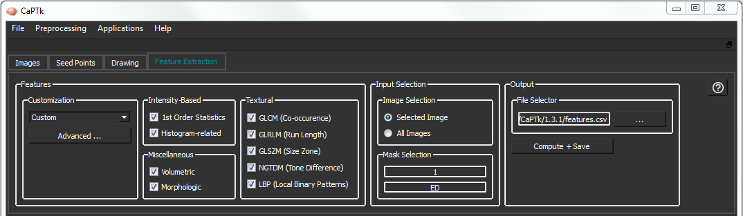
The feature extraction tab in CaPTk enables clinicians and other researchers to easily extract feature measurements, commonly used in image analysis, and conduct large-scale analyses in a repeatable manner. Although the feature panel in CaPTk is continuously expanding, it currently comprises i) intensity-based, ii) textural, and iii) volumetric/morphologic features.

The specialized applications in CaPTk, such as the EGFRvIII Surrogate Index, Survival Prediction, Recurrence Estimator, and SBRT-Lung use features of this panel. The general idea is to keep the features generic and adaptable for different types of medical images by just changing the input parameters. For now we provide some pre-selected parameters for Neuro and Torso images (i.e., Brain, Breast, Lung). Users can alter these pre-selected values through the Custom menu option, or create their own set of parameters via the Advanced menu. The output of the feature extraction tab can be either a .csv or an .xml file, with feature names and values. The table below gives details about the currently available features. Note that the reported features are extracted per modality, per annotated region and per offset (offset represents the radius around the center pixel; for radius 1, the offset will be +/- 1) value.

In the visualization panes, the "Z" axis is the center; and "Y" and "X" are to its left and right, respectively. "Z" represents the Axial view for RAI-to-LPS images.

Feature Panel screenshot

Feature Family	Specific Features	Parameter Name	Range	Default	Description, Formula and Comments
First Order Statistics	Minimum Maximum Mean Standard Deviation Variance Skewness Kurtosis	N.A.	N.A.	N.A.	Minimum Intensity = \( Min (I_{k}). \) where \( I_{k} \) is the intensity of pixel or voxel at index k. Maximum Intensity = \( Max (I_{k}). \) where \( I_{k} \) is the intensity of pixel or voxel at index k. Mean= \( \frac{\sum(X_{i})}{N} \) where N is the number of voxels/pixels. Standard Deviation = \( \sqrt{\frac{\sum(X-\mu)^{2}}{N}}\) where \(\mu\) is the mean of the data. Variance = \( \frac{\sum(X-\mu)^{2}}{N} \) where \(\mu\) is the mean intensity. Skewness = \( \frac{\sum_{i=1}^{N}(X_{i} - \bar{X})^{3}/N} {s^{3}} \) where \(\bar{X}\) is the mean, s is the standard deviation and N is the number of pixels/voxels. Kurtosis = \( \frac{\sum_{i=1}^{N}(X_{i} - \bar{X})^{4}/N}{s^{4}} \) where \(\bar{X}\) is the mean, s is the standard deviation and N is the number of pixels/voxels.
Histogram -based	Bin Frequency	Num_Bins	N.A.	10	Uses number of bins as input and the number of pixels in each bin would be the output.
Volumetric	Volume/Area	Dimensions Axis	2D:3D x,y,z	3D z	Volume/Area (depending on image dimension) and number of voxels/pixels in the ROI.
Morphologic	Elongation Perimeter Roundness Eccentricity	Dimensions Axis	2D:3D x,y,z	3D z	Elongation = \( \sqrt{\frac{i_{2}}{i_{1}}} \) where i_{n} are the second moments of particle around its principal axes. Perimeter = \( 2 \pi r \) where r is the radius of the circle enclosing the shape. Roundness = \( As/Ac = (Area of a shape)/(Area of circle) \) where circle has the same perimeter. Eccentricity = \( \sqrt{1 - \frac{a*b}{c^{2}}} \) where c is the longest semi-principal axis of an ellipsoid fitted on an ROI, and a and b are the 2nd and 3rd longest semi-principal axes of the ellipsoid.
Local Binary Pattern (LBP)		Radius Neighborhood	N.A. 2:4:8	N.A. 8	The LBP codes are computed using N sampling points on a circle of radius R and using mapping table.
Grey Level Co-occurrence Matrix (GLCM)	Energy Contrast Entropy Homogeneity Correlation Variance SumAverage Variance Auto Correlation	Num_Bins Num_Directions Radius Dimensions Offset Axis	N.A. 3:13 N.A. 2D:3D Average/Individual x,y,z	10 13 2 3D Average z	For a given image, a Grey Level Cooccurrence Matrix is created and \( g(i,j) \) represents an element in matrix Energy = \( \sum_{i,j}g(i, j)^2 \) Contrast = \( \sum_{i,j}(i - j)^2g(i, j) \) Entropy = \( -\sum_{i,j}g(i, j) \log_2 g(i, j) \) Homogeneity = \( \sum_{i,j}\frac{1}{1 + (i - j)^2}g(i, j) \) Correlation = \( \sum_{i,j}\frac{(i - \mu)(j - \mu)g(i, j)}{\sigma^2} \) Sum Average = \( \sum_{i,j}i \cdot g(i, j) = \sum_{i,j}j \cdot g(i, j)\)(due to matrix summetry) Variance = \( \sum_{i,j}(i - \mu)^2 \cdot g(i, j) = \sum_{i,j}(j - \mu)^2 \cdot g(i, j)\) (due to matrix summetry) AutoCorrelation = \(\frac{\sum_{i,j}(i, j) g(i, j)-\mu_t^2}{\sigma_t^2}\) where \(\mu_t\) and \(\sigma_t\) are the mean and standard deviation of the row (or column, due to symmetry) sums. All features are estimated within the ROI in an image, considering 26-connected neighboring voxels in the 3D volume.
Grey Level Run-Length Matrix (GLRLM)	SRE LRE GLN RLN LGRE HGRE SRLGE SRHGE LRLGE LRHGE	Num_Bins Num_Directions Radius Dimensions Axis Offset Distance_Range	N.A. 3:13 N.A. 2D:3D x,y,z Average/Individual 1:5	10 13 2 3D z Average 1	For a given image, a run-length matrix \( P(i; j)\) is defined as the number of runs with pixels of gray level i and run length j. Short Run Emphasis (SRE) = \( \frac{1}{n_r}\sum_{i,j}^{N}\frac{p(i,j)}{j^2} \) Long Run Emphasis (LRE) = \( \frac{1}{n_r}\sum_{j}^{N}p(i,j) \cdot j^2\) Grey Level Non-uniformity (GLN) = \( \frac{1}{n_r}\sum_{i}^{M}\Big(\sum_{j}^{N}p(i,j) \Big)^2 \) Run Length Non-uniformity (RLN) = \( \frac{1}{n_r}\sum_{j}^{N}\Big(\sum_{i}^{M}p(i,j) \Big)^2 \) Low Grey-Level Run Emphasis (LGRE)= \( \frac{1}{n_r}\sum_{i}^{M}\frac{p_g(i)}{i^2} \) High Grey-Level Run Emphasis (HGRE)= \( \frac{1}{n_r}\sum_{i}^{M}p_g(i) \cdot i^2 \) Short Run Low Grey-Level Emphasis (SRLGE)= \(\frac{1}{n_r}\sum_{i}^{M}\sum_{j}^{N}\frac{p(i,j)}{i^2 \cdot j^2} \) Short Run High Grey-Level Emphasis (SRLGE) = \( \frac{1}{n_r}\sum_{i}^{M}\sum_{j}^{N}\frac{p(i,j) \cdot i^2 }{j^2}\) Long Run Low Grey-Level Emphasis (LRLGE) = \( \frac{1}{n_r}\sum_{i}^{M}\sum_{j}^{N}\frac{p(i,j) \cdot j^2 }{i^2} \) Long Run High Grey-Level Emphasis (LRHGE) = \( \frac{1}{n_r}\sum_{i}^{M}\sum_{j}^{N}p(i,j) \cdot i^2 \cdot j^2 \) All features are estimated within the ROI in an image, considering 26-connected neighboring voxels in the 3D volume.
Neighborhood Grey-Tone Difference Matrix (NGTDM)	Coarseness Contrast Busyness Complexity Strength	Num_Bins Num_Directions Dimensions Axis Distance_Range	N.A. 3:13 2D:3D x,y,z 1:5	10 13 3D N.A. 1	Coarseness = \( \Big[ \epsilon + \sum_{i=0}^{G_{k}} p_{i}s(i) \Big]\) Contrast = \( \Big[\frac{1}{N_{s}(N_{s}-1)}\sum_{i}^{G_{k}}\sum_{j}^{G_{k}}p_{i}p_{j}(i-j)^2\Big]\Big[\frac{1}{n^2}\sum_{i}^{G_{k}}s(i)\Big] \) Busyness = \( \Big[\sum_{i}^{G_{k}}p_{i}s(i)\Big]\Big/ \Big[\sum_{i}^{G_{k}}\sum_{j}^{G_{k}}i p_{i} - j p_{j}\Big] \) Complexity = \( \sum_{i}^{G_{k}}\sum_{j}^{G_{k}} \Big[ \frac{(\|i-j\|)}{(n^{2}(p_{i}+p_{j}))} \Big] \Big[ p_{i}s(i)+p_{j}s(j) \Big]\) Strength = \( \Big[\sum_{i}^{G_{k}}\sum_{j}^{G_{k}}(p_{i}+p_{j})(i-j)^{2}\Big]/\Big[\epsilon + \sum_{i}^{G_{k}} s(i)\Big]\) Where \(p_{i}\) is the probability of occurrence of a voxel of intensity i and \(s(i)\) represents the NGTDM value of intensity i calculated as: \( \sum │i - Ai│\). Ai indicates the average intensity of the surrounding voxels without including the central voxel.
Grey Level Size-Zone Matrix (GLSZM)	SZE LZE GLN ZSN ZP LGZE HGZE SZLGE SZHGE LZLGE LZHGE GLV ZLV	Num_Bins Num_Directions Radius Dimensions Axis Distance_Range	N.A. 3:13 N.A. 2D:3D x,y,z 1:5	10 13 2 3D z 4	For a given image, a run-length matrix \( P(i; j)\) is defined as the number of runs with pixels of gray level i and run length j. Small Zone Emphasis (SZE) = \( \frac{1}{n_r}\sum_{i,j}^{N}\frac{p(i,j)}{j^2} \) Large Zone Emphasis(LZE) = \( \frac{1}{n_r}\sum_{j}^{N}p(i,j) \cdot j^2\) Gray-Level Nonuniformity (GLN) = \( \frac{1}{n_r}\sum_{i}^{M}\Big(\sum_{j}^{N}p(i,j) \Big)^2 \) Zone-Size Nonuniformity (ZSN) = \( \frac{1}{n_r}\sum_{j}^{N}\Big(\sum_{i}^{M}p(i,j) \Big)^2 \) Zone Percentage (ZP) = \( \frac{n_{r}}{n_p} \) where \( n_r \) is the total number of runs and \( n_p \) is the number of pixels in the image. Low Grey-Level Zone Emphasis (LGZE)= \( \frac{1}{n_r}\sum_{i}^{M}\frac{p_g(i)}{i^2} \) High Grey-Level Zone Emphasis (HGZE)= \( \frac{1}{n_r}\sum_{i}^{M}p_g(i) \cdot i^2 \) Short Zone Low Grey-Level Emphasis (SZLGE)= \(\frac{1}{n_r}\sum_{i}^{M}\sum_{j}^{N}\frac{p(i,j)}{i^2 \cdot j^2} \) Short Zone High Grey-Level Emphasis (SZLGE) = \( \frac{1}{n_r}\sum_{i}^{M}\sum_{j}^{N}\frac{p(i,j) \cdot i^2 }{j^2}\) Long Zone Low Grey-Level Emphasis (LZLGE) = \( \frac{1}{n_r}\sum_{i}^{M}\sum_{j}^{N}\frac{p(i,j) \cdot j^2 }{i^2} \) Long Zone High Grey-Level Emphasis (LZHGE) = \( \frac{1}{n_r}\sum_{i}^{M}\sum_{j}^{N}p(i,j) \cdot i^2 \cdot j^2 \) All features are estimated within the ROI in an image, considering 26-connected neighboring voxels in the 3D volume.

REQUIREMENTS:

An image or a set of co-registered images
An ROI set containing masks of various labels, for which features will be extracted. If an ROI set is not provided, features can be calculated for the entire image.

USAGE:

Load image(s) and an ROI set (if an ROI set is not available, the user can draw a mask using any label).
Select the type of features to extract from the drop-down menu:
- SBRT_Lung: the feature definition provided by CBICA which have been used to generate features for SBRT_Lung
- Custom: manually selected & customized features
Use the Advanced button to parameterize the selected features.
Select the image to extract features from, or select All Images under the Image Selection dialog to extract features for all the images that have been loaded in CaPTk.
The user has the option to extract features only for specific labels included in the loaded ROI (default behavior is feature extraction for all labels). Number of request labels for feature extraction should match up with their respective names.
Click on browse button and provide a location for the CSV (or XML) output file.
Use the Advanced button to parameterize the selected features.
Click compute.
The results are saved in the specified file.

Next (Building from source)

Functionality/Usage Details
Generated on Tue Feb 6 2018 10:02:06 for Cancer Imaging Phenomics Toolkit (CaPTk) by 1.8.14