Contents:
- EGFRvIII Surrogate Index (PHI Estimator)
- Glioblastoma Infiltration Index (Recurrence)
- Survival Index Prediction
- Confetti
- WhiteStripe
- Radiomics Analysis of Lung Cancer using Stereotactic Body Radiation Therapy (SBRT Lung)
- Directionality Estimation
- LIBRA
EGFRvIII Surrogate Index (PHI Estimator)
This application evaluates the Epidermal Growth Factor Receptor version III (EGFRvIII) status in primary glioblastoma patients, by quantitative pattern analysis of the spatial heterogeneity of peritumoral perfusion dynamics from Dynamic Susceptibility Contrast (DSC) MRI scans, through the Peritumoral Heterogeneity Index (PHI / φ-index) [1,2].
REQUIREMENTS:
- Post-contrast T1-weighted (T1-Gd): To annotate the immediate peritumoral ROI.
- T2-weighted Fluid Attenuated Inversion Recovery (T2-FLAIR): To annotate the distant peritumoral ROI.
- Dynamic susceptibility contrast-enhanced MRI (DSC-MRI): To perform the analysis and extract the PHI.
USAGE:
- Annotate 2 ROIs: one near (label 1) the enhancing tumor and another far (label 2) from it (but still within the peritumoral region).
- Once the 2 ROIs are annotated, the application can be launched by using the menu option: 'Applications -> EGFRvIII Surrogate Index'.
- A pop-up window appears displaying the results (within <1 minute).
- This application is also available as with a stand-alone CLI for data analysts to build pipelines around.
Glioblastoma Infiltration Index (Recurrence)
This presents the imaging signatures of deeply infiltrating tumor which largely agree with subsequent recurrence in de novo glioblastoma patients, via multi-parametric MRI analysis that assesses the spatial heterogeneity of peritumoral edema. [3,4]
REQUIREMENTS:
- T1-weighted (T1)
- Post-contrast T1-weighted (T1-Gd)
- T2-weighted (T2)
- T2-weighted Fluid Attenuated Inversion Recovery (T2-FLAIR)
- Diffusion Tensor Imaging (DTI) derivative measurements: Axial Diffusivity (AX), Fractional Anisotropy (FA), Radial Diffusivity (RAD), Apparent Diffusion Coefficient (ADC)
- Dynamic Susceptibility Contrast-Enhanced (DSC) MRI
- Segmentation of tumor in one image: Non-enhancing tumor core (Label=175), Enhancing tumor core (Label=200)
- The data for each patient should be organized in the following directory structure.
- SubjectID
- CONVENTIONAL
- "my_T1_file.nii.gz"
- "my_T2_file.nii.gz"
- "my_T1CE_file.nii.gz"
- "my_FLAIR_file.nii.gz"
- DTI
- "my_AX_file.nii.gz"
- "my_FA_file.nii.gz"
- "my_RAD_file.nii.gz"
- "my_TR_file.nii.gz"
- PERFUSION
- "my_PERFUSION_file.nii.gz"
- SEGMENTATION
- "my_segmentation_file.nii.gz"
- "my_near_region_file.nii.gz" (only for training a new model)
- "my_far_region_file.nii.gz" (only for training a new model)
- CONVENTIONAL
- SubjectID
USAGE:
- Preparing a new Recurrence Estimation model:
- The data for multiple patients should be organized in the above mentioned structure and be copied in one directory, let's say "TrainingData".
- TrainingData
- SubjectID1
- SubjectID2
- ...
- SubjectIDn
- Once the data is organized, the application can be launched by using the menu option: 'Applications -> Glioblastoma Infiltration Index'.
- A pop-up dialog opens up showing the recurrence panel.
- Select the input directory (TrainingData).
- Select the output directory where user wants to save the prepared model and click on 'Confirm'.
- System loads all the qualified subjects, which adhere to the organization structure and have all the data available, and prepares a model.
- A pop-up window appears displaying the completion of model building (time depends on the number of training subjects. ~1.5*TrainingSubejcts minutes).
- This application is also available as with a stand-alone CLI for data analysts to build pipelines around.
- Recurrence Estimation on an existing model:
- The data for multiple patients should be organized in the above mentioned structure and be copied in one directory, let's say "TestData".
- TestData
- SubjectID1
- SubjectID2
- ...
- SubjectIDn
- Once the data is organized, the application can be launched by using the menu option: 'Applications -> Glioblastoma Infiltration Index'.
- A pop-up dialog opens up showing the recurrence panel.
- Select the input directory (TestData).
- Select the model directory. A model prepared on a large cohort of HUP is already present in CaPTk package. In order to use this model, select ../Data/recurrence folder. Otherwise, users can use their own model.
- Select the output directory where user wants to save the infiltration maps and click on 'Confirm'.
- System loads all the qualified subjects, which adhere to the organization structure and have all the data available, and computes infiltration maps.
- A pop-up window appears displaying the completion of infiltration map calculation (time depends on number of test subjects. ~1.5*TestSubejcts minutes).
- This application is also available as with a stand-alone CLI for data analysts to build pipelines around.
- Recurrence Estimation on a loaded case (patient):
- Load all the required images for the given patient.- The patient data does not need to adhere to the directory structure. It can be loaded in the system from anywhere.
- Select the file type of each image from the image tab.
- Annotate 3 ROIs: one near (label 1) the enhancing tumor, one far (label 2) from it (but still within the peritumoral region) and another within tumor (label 3).
- Once the ROIs are initialized, the application can be launched by using the menu option: 'Applications -> Glioblastoma Infiltration Index'.
- A pop-up dialog opens up showing the recurrence panel.
- Select output directory and click on 'Confirm'.
- A pop-up window appears displaying the results (within ~3 minutes).
Survival Index Prediction
This presents a survival prediction index (SPI) by using multi-parametric MRI (before first surgery) analysis of de novo glioblastoma patients. The predicted survival indices largely agree with subsequent real survival of patients. [5]
REQUIREMENTS:
- T1-weighted (T1)
- Post-contrast T1-weighted (T1-Gd)
- T2-weighted (T2)
- T2-weighted Fluid Attenuated Inversion Recovery (T2-FLAIR)
- Diffusion Tensor Imaging (DTI) derivative measurements: Axial Diffusivity (AX), Fractional Anisotropy (FA), Radial Diffusivity (RAD), Apparent Diffusion Coefficient (ADC)
- Dynamic susceptibility contrast-enhanced (DSC) MRI measurements: DSC-PSR (Percent Signal Recovery), DSC-RCBV (Relative Cerebral Blood Volume), DSC-PH (Peak Height)
- Segmentation of three tumor partitions in one image: Edema (Label=100), Non-enhancing tumor core (Label=175), Enhancing tumor core (Label=200)
- Feature file: A csv file having patient's demographics. Should have age (in first column) and survival (in second column) for training a new model, and age only for survival prediction of new patients.
- The data for each patient should be organized in the following directory structure.
- SubjectID
- features.csv file
- CONVENTIONAL
- "my_T1_file.nii.gz"
- "my_T2_file.nii.gz"
- "my_T1CE_file.nii.gz"
- "my_FLAIR_file.nii.gz"
- DTI
- "my_AX_file.nii.gz"
- "my_FA_file.nii.gz"
- "my_RAD_file.nii.gz"
- "my_TR_file.nii.gz"
- PERFUSION
- "my_RCBV_file.nii.gz"
- "my_PSR_file.nii.gz"
- "my_PH_file.nii.gz"
- SEGMENTATION
- "original_segmentation_file.nii.gz"
- "segmentation_file_in_atlas_space.nii.gz"
- SubjectID
USAGE:
- Preparing a new Survival Prediction model:
- The data for multiple patients should be organized in the above mentioned structure and be copied in one directory, let's say "TrainingData".
- TrainingData
- SubjectID1
- SubjectID2
- ...
- SubjectIDn
- Once the data is organized, the application can be launched by using the menu option: 'Applications -> Survival Prediction Index'.
- A pop-up dialog opens up showing the survival panel.
- Select the input directory (TrainingData).
- Select the output directory where user wants to save the prepared model and click on 'Confirm'.
- System loads all the qualified subjects, which adhere to the organization structure and have all the data available, and prepares a model.
- A pop-up window appears displaying the completion of model building (time depends on the number of training subjects. ~2*TrainingSubejcts minutes).
- This application is also available as with a stand-alone CLI for data analysts to build pipelines around.
- Survival Prediction on an existing model:
- The data for multiple patients should be organized in the above mentioned structure and be copied in one directory, let's say "TestData".
- TestData
- SubjectID1
- SubjectID2
- ...
- SubjectIDn
- Once the data is organized, the application can be launched by using the menu option: 'Applications -> Survival Prediction Index'.
- A pop-up dialog opens up showing the survival panel.
- Select the input directory (TestData).
- Select the model directory. A model prepared on a large cohort of HUP is present in CaPTk package. In order to use this model, select ../Data/survival folder. Otherwise, users can select their own model.
- Select the output directory where user wants to save the SPI in .csv file format and click on 'Confirm'.
- System loads all the qualified subjects, which adhere to the organization structure and have all the data available, and computes SPI.
- A pop-up window appears displaying the completion of SPI calculation. The window will also show SPI index if there is only one subject in TestData. (time depends on number of test subjects. ~2*TestSubejcts minutes).
- This application is also available as with a stand-alone CLI for data analysts to build pipelines around.
Confetti
This is a method for automated extraction of white matter tracts of interest in a consistent and comparable manner over a large group of subjects without drawing the inclusion and exclusion regions of interest (ROI), facilitating an easy correspondence between different subjects, as well as providing a representation that is robust to edema, mass effect, and tract infiltration [8-10]. Confetti includes three main steps:
- Connectivity signature generation for fibers
- Clustering of fibers using a mixture of multinomials (MNs) clustering method and Expectation-Maximization (EM) optimization framework
- Extraction of predefined white matter tracts.
REQUIREMENTS:
- Fiber set (Streamline) to be clustered: The fiber set can be generated using any tractography model, but the current version requires the file to be saved in the ".Bfloat format" (i.e. fiber format of Camino package). Different converters can be be used to convert .trk to .Bfloat and vice-versa.
- Track Density Images (TDI): When using GUI, it needs to be generated in the manner explained below; this constraint is not present when using Confetti via the command line.
- Parcellation of the brain into 87 Desikan/Freesurfer gray matter (GM) regions [11]
Generation of TDI Images with GUI:
- Freesurfer [11] is used with the Desikan atlas [12] to define 87 gray matter ROIs in the user diffusion space.
- Region IDs of the ROIs as used by Freesurfer is provided in the example file "{CaPTk_Sample_Data}/Confetti/input/freesurfer_ROIs.csv".
- TDIs must be generated using the probtrackx utility of FSL package [13] with its default parameters and 5000 seeds per voxel.
- Each TDI image is a whole brain voxel-map, with each voxel having the number of fibers passing through this voxel and reaching to one of the 87 gray matter ROIs defined by Freesurfer.
- In total, you should have 87 TDI, each corresponding to one ROI.
USAGE:
- Open Confetti UI using the 'Applications -> Confetti' menu option.
- Load the required images using "Streamline File" and "TDI Directory".
- Specify the output directory and click on 'Run Confetti'.
- Visually review the output tracks by double clicking respective fields on the populated list view.
WhiteStripe
This algorithm normalizes conventional MRI [14] by detecting a latent subdistribution of normal tissue and linearly scaling the histogram of images.
REQUIREMENTS:
- Bias-corrected (N3 or N4) T1-weighted or T2-weighted images, ideally either skull-stripped or rigidly aligned to MNI space.
USAGE:
- Launch the WhiteStripe UI using the 'Applications -> WhiteStripe' menu option.
- Specify the Input and Output files and different parameters (defaults are populated).
- Click on 'Run WhiteStripe" and the results can be seen in a slice format using "Toggle Mask/Image" checkbox.
- Use 'Level Display' when needed.
- Batch Processing can be done using similar options under the specific tab.
NOTE: WhiteStripe uses KernelFit library from Lentner.
Radiomics Analysis of Lung Cancer (SBRT Lung)
This application calculates quantitative imaging measures including Intensity statistics, Gray Level Co-occurrence Matrix (GLCM), Gray Level Run-Length Matrix (GLRLM), Local Binary Patterns (LBPs), and shape features from PET/CT scans of lung cancer patients for predicting clinical outcomes, such as treatment response and patient survival using pattern recognition and machine learning techniques [15]. It consists of 2 steps: 'Segment' and 'Analyze'.
REQUIREMENTS:
- CT image
- PET image (co-registered to the CT image)
USAGE:
- Once the images have been loaded, click on 'SBRT Segment' from the 'Applications' menu.
- The mask is automatically loaded. Please correct the mask as required (it should ideally cover the lesions in the lung).
- Click on 'SBRT Analyze' from the 'Applications' menu.
- The prediction result comes up in a pop-up box.
NOTE: SBRT uses a pre-trained model for estimation; in the future we will provide a mechanism to do training on own data.
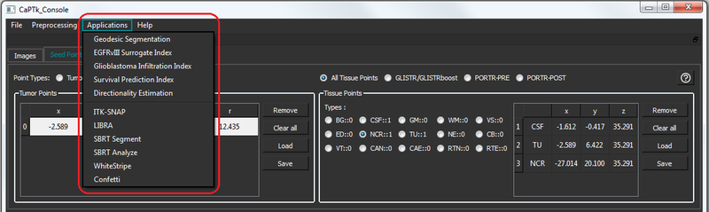
Directionality Estimation
REQUIREMENTS:
- Input image
- Input ROI which has at least 1 label
USAGE:
- Place a tissue point with label TU from where the measurements are needed
- Select "Applications > Directionality Estimation" from the menu
- Pop-up box shows coordinates along the different planes
- Tissue point table gets updated with 3 points marked "CSF" (which are correspond to the direction of max point along the different planes) and 1 point marked "RTN" (which is the actual point of max distance from initialized seed point)
- The user has the option to either save the result in a text file in a location of their choosing or ignore and run the algorithm again.
LIBRA
LIBRA is a stand-alone software application for fully-automated breast density segmentation. LIBRA is based on a published algorithm [16] that works on either raw (i.e., “FOR PROCESSING”) or vendor post-processed (i.e., “FOR PRESENTATION”) digital mammography images from two vendors (GE Healthcare and Hologic) and it generates quantitative estimates of breast area, dense area and breast percent density.
Within CaPTk specifically, LIBRA is available via an easy-to-use interactive mode with Graphical-User-Interface where the user is prompted to select either a single DICOM image or a folder of DICOM images, an output folder for the results, and whether they wish to save intermediate files. All results are stored in the output folder defined by the user.
Please see the LIBRA manual for detailed instructions: http://www.med.upenn.edu/sbia/libra.html
References:
[1] S.Bakas, H.Akbari, J.Pisapia, M.Rozycki, D.M.O'Rourke, C.Davatzikos. "Identification of Imaging Signatures of the Epidermal Growth Factor Receptor Variant III (EGFRvIII) in Glioblastoma", Neuro-Oncology, 17(Suppl.5):V154, 2015, DOI: 10.1093/neuonc/nov225.05
[2] S.Bakas, H.Akbari, J.Pisapia, M.Martinez-Lage, M.Rozycki, S.Rathore, N.Dahmane, D.M.O'Rourke, C.Davatzikos. "In vivo detection of EGFRvIII in glioblastoma via perfusion magnetic resonance imaging signature consistent with deep peritumoral infiltration: the φ-index", Clinical Cancer Research, 2017 DOI: 10.1158/1078-0432.CCR-16-1871
[3] H.Akbari, L.Macyszyn, X.Da, M.Bilello, R.L.Wolf, M.Martinez-Lage, G.Biros, M.Alonso-Basanta, D.M.O'Rourke, C.Davatzikos. "Imaging Surrogates of Infiltration Obtained Via Multiparametric Imaging Pattern Analysis Predict Subsequent Location of Recurrence of Glioblastoma", Neurosurgery, 2016 Apr 1; 78(4):572-80.
[4] H.Akbari, L.Macyszyn, X.Da, M.Bilello, R.Verma, D.M.O'Rourke, C.Davatzikos. "Pattern analysis of dynamic susceptibility contrast-enhanced MR imaging demonstrates peritumoral tissue heterogeneity", Radiology, 2014 Jun 19;273(2):502-10.
[5] L.Macyszyn, H.Akbari, J.M.Pisapia, X.Da, M.Attiah, V.Pigrish, Y.Bi, S.Pal, R.V.Davuluri, L.Roccograndi, N.Dahmane. "Imaging patterns predict patient survival and molecular subtype in glioblastoma via machine learning techniques", Neuro-oncology, 2016 Mar 1;18(3):417-25.
[6] H.Akbari, L.Macyszyn, X.Da, R.L.Wolf, M.Bilello, R.Verma, D.M.O'Rourke, C.Davatzikos, "Pattern analysis of dynamic susceptibility contrast-enhanced MR imaging demonstrates peritumoral tissue heterogeneity", Radiology, 2014 Jun 19;273(2):502-10.
[7] H.Akbari, L.Macyszyn, J.Pisapia, X.Da, M.Attiah, Y.Bi, S.Pal, R.Davuluri, L.Roccograndi, N.Dahmane, R.Wolf, M.Bilello, D.M.O'Rourke, C.Davatzikos, "Survival Prediction in Glioblastoma Patients Using Multi-parametric MRI Biomarkers and Machine Learning Methods", American Society of Neuroradiology, 2015; O-525, pp. 2042-2044 (http://www.asnr.org/sites/default/files/proceedings/2015_Proceedings.pdf)
[8] B.Tunç, M.Ingalhalikar, W.A.Parker, J.Lecoeur, R.L.Wolf, L.Macyszyn, S.Brem, R.Verma, "Individualized Map of White Matter Pathways: Connectivity-based Paradigm for Neurosurgical Planning", Neurosurgery, 2016; Vol. 79 (4), pp. 568-77.
[9] B.Tunç, W.A.Parker, M.Ingalhalikar, R.Verma, "Automated tract extraction via atlas based Adaptive Clustering", NeuroImage, 2014; Vol. 102 (2), pp. 596-607.
[10] B.Tunç, A.R.Smith, D.Wasserman, X.Pennec, W.M.Wells, R.Verma, K.M.Pohl, "Multinomial Probabilistic Fiber Representation for Connectivity Driven Clustering", Information Processing in Medical Imaging (IPMI), 2013.
[11] B.Fischl, M.I.Sereno, A.M.Dale, "Cortical surface-based analysis. II: Inflation, flattening, and a surface-based coordinate system", NeuROImage, 1999; 9:195–207.
[12] R.S.Desikan, F.Segonne, B.Fischl, B.Quinn, B.Dickerson, D.Blacker, R.Buckner, A.Dale, R.Maguire, B.Hyman, M.Albert, R.Killiany, "An automated labeling system for subdividing the human cerebral cortex on MRI scans into gyral based regions of interest", NeuROImage, 2006; 31.
[13] M.Jenkinson, C.F.Beckmann, T.E.J.Behrens, M.W.Woolrich, S.M.Smith, "FSL", NeuROImage, 2012; 62:782–790.
[14] R.T.Shinohara, E.M.Sweeney, J.Goldsmith, et al., "Statistical normalization techniques for magnetic resonance imaging", NeuROImage Clinical, 2014.
[15] H.Li, M.Galperin-Aizenberg, D.Pryma, C.Simone, Y.Fan, "Predicting treatment response and survival of early-stage non-small cell lung cancer patients treated with stereotactic body radiation therapy using unsupervised two-way clustering of radiomic features", International Workshop on Pulmonary Imaging, 2017.
[16] B.M.Keller, D.L.Nathan, Y.Wang, Y.Zheng, J.C.Gee, E.F.Conant, and D.Kontos, "Estimation of breast percent density in raw and processed full field digital mammography images via adaptive fuzzy c-means clustering and support vector machine segmentation", Medical Physics 39 (8), 4903-4917
- Generated on Tue Feb 6 2018 10:02:06 for Cancer Imaging Phenomics Toolkit (CaPTk) by
 1.8.14